AB-025
Using SPICE To Model DC Motors
Introduction
SPICE (Simulation Program with Integrated Circuit Emphasis) is an open-source program for simulating electrical circuits. It enables engineers to model the behaviour of their circuits in software, which reduces prototyping costs and time.
As DC motors have mechanical properties – i.e. they cannot be simulated accurately only considering electrical properties – it can be difficult to use them in SPICE. This Application Bulletin guides you through the principle of operation and extends the DC motor model for vibration motors and gear motors.
Principles Of Operation
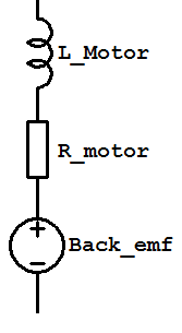
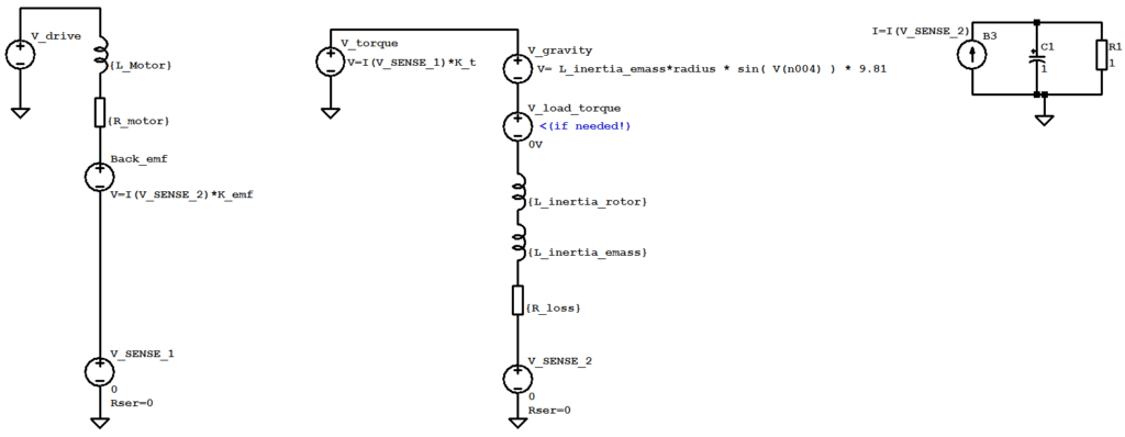
The equivalent circuit for a DC motor consists of an inductor, a resistor and a voltage source in series. These represent the coil inductance, coil resistance, and back EMF respectively.

Get in touch
Speak to a member of our team.
Motor catalogue
Looking for our products?
Reliable, cost-effective miniature mechanisms and motors that meet your application demands.
The back EMF voltage source is dependent on the speed of the motor and the torque constant Kτ. W, therefore, need a mechanical system model in order to calculate the speed of the motor. The SPICE engine doesn’t explicitly support mechanical models, however, it is facilitated by the use of electrical equivalent circuits.
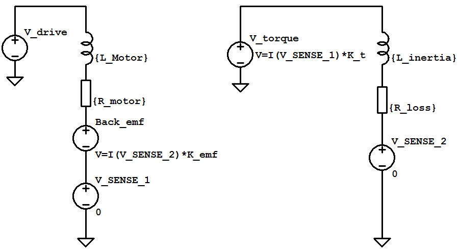
Example parameters for the circuit:
.PARAM K_t = 900u
.PARAM K_EMF = 900u
.PARAM L_Motor = 50u
.PARAM R_motor = 5.5
.PARAM R_loss = 300n
.PARAM L_inertia = 15n
Current-dependent voltage sources are used to communicate information between the electrical and mechanical equivalent circuits. Note the two 0V voltage sources, V_sense_1 and V_sense_2. These do not alter the behaviour of the circuit and are simply used to provide convenient current measurements. The back EMF voltage source depends on the current sensed by V_Sense_2.
Justification For The Mechanical Equivalent Circuit
The table below outlines the variables in the mechanical circuit.
| Electrical Variabledescription, symbol, unit | Mechanical Equivalentdescription, symbol, unit |
| Voltage, V, [V] ≡ [kg⋅m2⋅A^-1⋅s^-3 ] | Torque, τ, [N⋅m] ≡ [kg⋅m2⋅s^-2] |
| Current, I, [A] | Angular velocity, ω, [rad⋅s^-1] |
| Resistance, R, [Ω] ≡ [kg⋅m2⋅A^-2⋅s^-3] | Coefficient of viscous friction, μ, [kg⋅m2⋅s^-1] |
| Inductance, L, [H] ≡ [kg⋅m2⋅A^-2⋅s^-2] | Moment of Inertia, I, [kg⋅m2] |
Important Note: We can see from the above that the Current and the Moment of Inertia share the same symbol, I. Pay careful attention to whether you’re working with the electrical or the mechanical parameters to avoid mistakes.
The rotor torque in a DC motor is determined by the current through the coils and the torque constant, Kτ. Torque is represented as the voltage V_torque in the mechanical equivalent circuit. The resulting speed of the rotor, ω, is represented by the current in the mechanical circuit.
So what limits the speed of the rotor? Anything in the mechanical circuit which limits the current, such as the resistor R_loss. The voltage dropped over R_loss depends on the current, as per Ohm’s law:𝑉=𝐼×𝑅
This acts to reduce the rotor torque, and it has a velocity-dependent loss. In other words, it represents velocity-dependent friction. The equivalent equation is:𝐹=𝜇×𝜔
Where μ is the coefficient of friction. This is a simple model of viscous friction (see more in the conclusion), and does not fully convey the complexities of friction in DC motors. It does, however, clearly illustrate the role of friction as an energy sink in the mechanical system which acts to reduce the speed of the motor.
What does the inductor represent? L_inertia limits the current in the mechanical circuit when there is a change in voltage V_torque. The voltage dropped across the motor is given (remember, here I is current):𝑉=–𝐿𝑑𝐼𝑑𝑡
The mechanical equivalent for which is (I now represents the moment of inertia):𝜏=𝐼×𝛼=𝐼×𝑑𝜔𝑑𝑡
Where 𝛼 is angular acceleration. It is therefore clear that in our model the inductance L_inertia is the electrical equivalent variable of the moment of inertia of the rotor.
Modelling The Transition To Steady State Behaviour
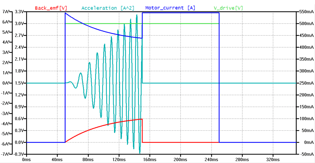
Assume initially that the motor is unpowered (V_drive = 0V). After some time, a DC voltage is applied (V_drive = 3V). This change in voltage causes a change of current in the circuit. The coil inductance opposes this change and generates a voltage proportional to dI/dt which is known as back EMF. This is observed as the gradient of the initial current inrush (the greater the inductance, the lower the rate of change, the shallower the gradient).
After the voltage is applied the motor begins to turn. The faster the motor turns, the greater the back EMF in the coils. This back EMF not only reduces the height of the initial current inrush but in the steady-state means that the current draw is significantly lower than the motor terminal resistance alone would permit. This can be proven with a quick calculation from the DC motor datasheet, such as the 106-002, by taking the Rated Voltage and dividing it by the Typical Terminal Resistance. For example, using the 106-002 we calculate 3𝑉16Ω=187.5𝑚𝐴, which is much higher than the Typical N/L current of 17mA – caused by the back EMF limiting the current flow.
The peak inrush current is identified as the first stationary point in the plot below (marker B). It is specified in our datasheets as “Max. Start Current”.
Note that the peak inrush current is limited by back EMF, which is a function of the motor speed. Therefore a finite drive signal rise time, say 10μs instead of 0μs, affects this value. Remember that an instant transition between voltages is not physical. In a real application, it can be useful to limit the rise time of the driving signal for just this reason.
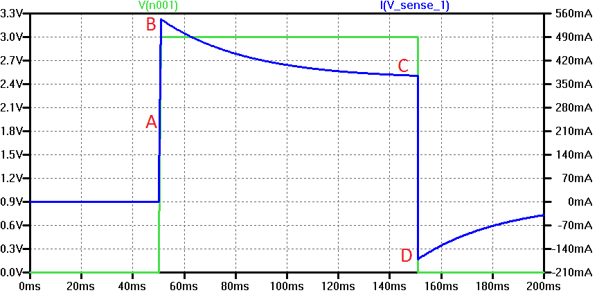
A – finite 𝑑𝐼𝑑𝑡 due to coil inductance
B – height of peak limited by back-EMF
C – current draw reaches steady-state value as back emf and friction balance
D – driving signal (green) terminated, large back emf spike
Note: that a large negative voltage spike at D as the motor coil inductance resists the changing current. These spikes are why flyback diodes are recommended (such as the Schottky flyback diode recommended here).
It can be seen that the coil inductance acts to limit the initial current inrush, whereas the back EMF acts to reduce the steady-state current. We can model a motor in a stall condition as a sudden large increase in the mechanical equivalent circuit resistance.
Determining Rotor Position
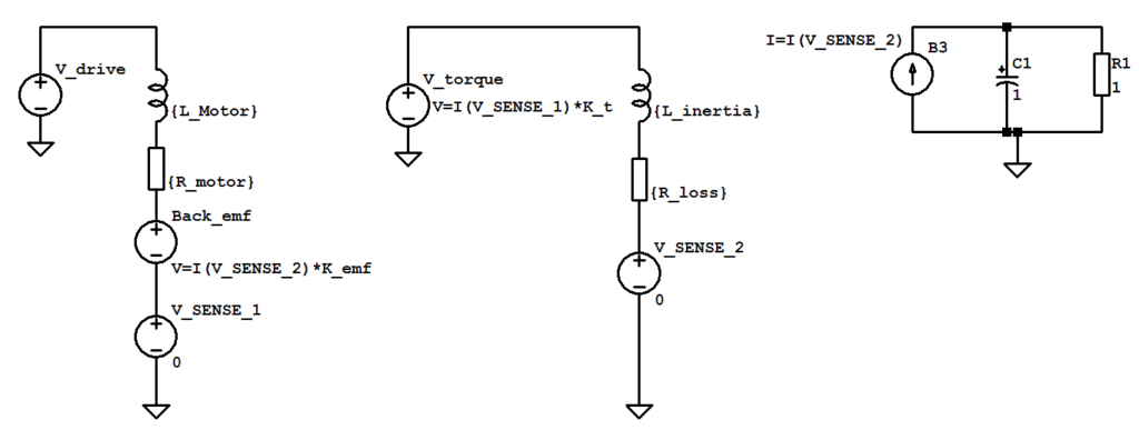
The voltage at C1 provides the angular position of the rotor in radians.
Modelling A Vibration Motor
We can use this simple DC motor to plot the periodic acceleration of a test sled caused by a vibration motor. We assume:
- a test sled of mass 100g
- an eccentric point mass of 5g at a radius of 2mm from the rotor axis
- the moment of inertia of the rotor to be negligible relative to the moment of inertia of the eccentric mass
- the mass of the motor to be negligible relative to the mass of the test sled
Considering the centripetal force of a mass rotating about a fixed point:𝐹=𝑚𝑒𝑐𝑐𝑒𝑛𝑡𝑟𝑖𝑐×𝑟×𝜔2
so along an axis, say x, this force is given by:𝐹𝑥=𝑚𝑒𝑐𝑐𝑒𝑛𝑡𝑟𝑖𝑐×𝑟×𝜔2𝑐𝑜𝑠(𝜃)
Where theta (𝜃) is the angular position of the rotor and r is the radius of the eccentric point mass.
By Newton’s second law, we set equation 4 equal to the magnitude force upon the test sled, mass m_sled:𝑚𝑒𝑐𝑐𝑒𝑛𝑡𝑟𝑖𝑐×𝑟×𝜔2=𝑚𝑠𝑙𝑒𝑑𝑎𝑠𝑙𝑒𝑑
or using equation 6 and equating forces along a given axis x:𝑚𝑒𝑐𝑐𝑒𝑛𝑡𝑟𝑖𝑐×𝑟×𝜔2𝑐𝑜𝑠(𝜃)=𝑚𝑠𝑙𝑒𝑑𝑎𝑠𝑙𝑒𝑑,𝑥
Rearranging for 𝑎𝑠𝑙𝑒𝑑,𝑥:𝑎𝑠𝑙𝑒𝑑,𝑥=𝑚𝑒𝑐𝑐𝑒𝑛𝑡𝑟𝑖𝑐⋅𝑟⋅𝜔2⋅𝑐𝑜𝑠(𝜃)𝑚𝑠𝑙𝑒𝑑,𝑥[𝑚⋅𝑠−2]
or in units of gravitational acceleration (where 𝑔=9.81[𝑚𝑠−2] ):𝑎𝑠𝑙𝑒𝑑,𝑥=𝑚𝑒𝑐𝑐𝑒𝑛𝑡𝑟𝑖𝑐⋅𝑟⋅𝜔2⋅𝑐𝑜𝑠(𝜃)9.81⋅𝑚𝑠𝑙𝑒𝑑,𝑥[𝑔]
Inserting the constants assumed earlier, the following trace is added to the LTSpice plot window:
.00001*I(V_sense_2)*I(V_sense_2)*sin(V(n003)*57.329)
where V(n003) is the voltage measured at the capacitor in the integrator circuit (the particular node value may well be different to this in your model), and I(V_sense_2) is the current measured in the mechanical equivalent circuit. By default, LTSpice computes trigonometric functions with arguments in degrees. Thus, the argument in Trace Equation 1 is converted from radians by the multiplication factor of 57.329 ( = 360/(2*pi) ) . An example of this trace output can be seen in the stall condition model extension.
Dimensional Analysis Of Equations 9 And 11
Using the table in figure 3, we can perform a dimensional analysis of the final equations in order to check their validity. Analysing the units of the right hand side of equation 9:[𝑚𝑒𝑐𝑐𝑒𝑛𝑡𝑟𝑖𝑐]⋅[𝑟]⋅[𝜔2]⋅𝑐𝑜𝑠(𝜃)[𝑚𝑠𝑙𝑒𝑑,𝑥]=𝑘𝑔⋅𝑚⋅𝑠−2𝑘𝑔=𝑚⋅𝑠−2
Which gives the expected result – the units are those of acceleration. What units would we expect to be displayed in the SPICE trace? Performing the same analysis on equation 11:.00001⋅𝐼(𝑉𝑠𝑒𝑛𝑠𝑒2)⋅𝐼(𝑉𝑠𝑒𝑛𝑠𝑒2)⋅𝑠𝑖𝑛(𝑉(𝑛003)⋅57.329)=[𝐴]⋅[𝐴]=[𝐴2]
As we have already included the gravitational constant and mass of the test sled in the multiplier “0.00001”, 1A2 in the trace window represents an acceleration of 1G, as normalised for a 100g test sled.
Behavioural Extensions To The Model
Extensions to the basic DC motor model are presented, with the intention of emulating the behaviour of real-world motors.
1) Separation Of Rotor/Eccentric Mass Inertia, Inclusion Of Gravity
The model below improves upon the earlier model by separating the inertia of the rotor and eccentric mass. Additional voltage sources are also included in the mechanical equivalent circuit, including a source to account for the effect of gravity on the eccentric mass. An optional load torque voltage source is also included.
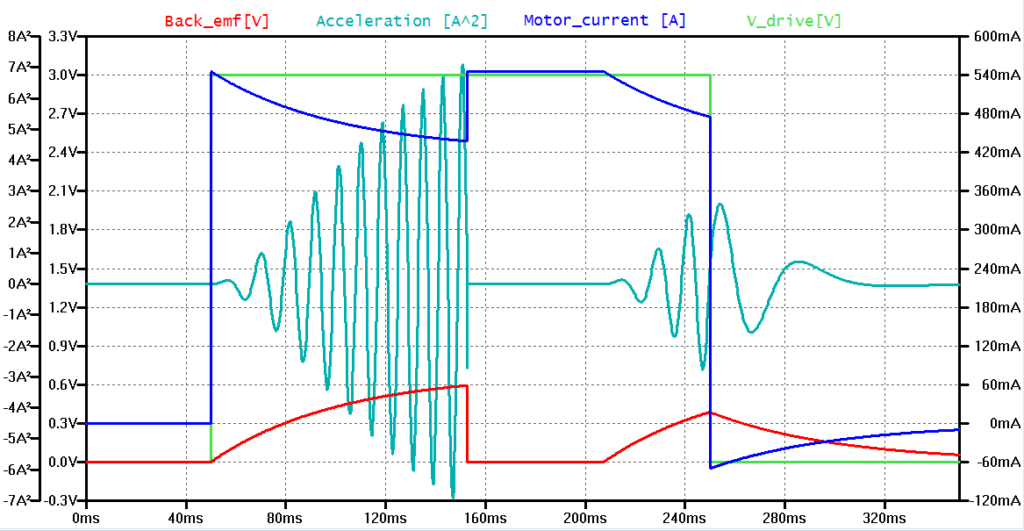
2) Non-Zero Turn-On Voltage
Gradually increase the driving voltage from 𝑉=0 to 𝑉=𝑉𝑟𝑎𝑡𝑒𝑑 on a real-life DC motor and it will exhibit a finite turn-on voltage. At this voltage, the current through the motor coils results in a sufficient torque to overcome the inertia and static friction of the system and the rotor begins to turn. This behaviour is exhibited in the “typical performance characteristics” plots on our vibration motor datasheets as an apparent discontinuity in motor speed.
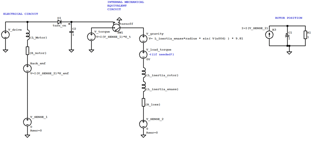
We define the forward voltage drop of a diode (D1) as 0.6V. Once V_drive exceeds this 0.6V limit, the diode conducts, and the voltage at A exceeds the threshold voltage of the voltage controlled switch. If the input V_drive drops below 0.7V at some later time, the voltage at A is clamped by C1, and thus this mechanical system remains unaffected by the static friction limit (which is correct, as the motor is moving). Example model parameters;
PULSE(0 3 100m 100m 100m 100m)
.tran 0 500m 0 1m
.model turnoff SW(Vt = 1u Ron = 1n)
.model turn_on D( Vfwd = 0.6 Rrev = 1n Ron = 1n)
3) Modelling A Reduction Gearbox
A gearbox is modelled by the inclusion of an additional mechanical equivalent circuit. The current from the “internal” mechanical circuit is measured and divided by the reduction gear ratio. This determines the speed at the shaft of the motor. Additional terms for friction and inertia are included, as well as a voltage source into which a load torque profile can be set.
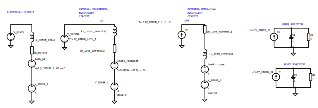
A “shaft feedback” voltage source is included in the internal mechanical circuit, the magnitude of which depends on the loading at the gearbox output shaft.
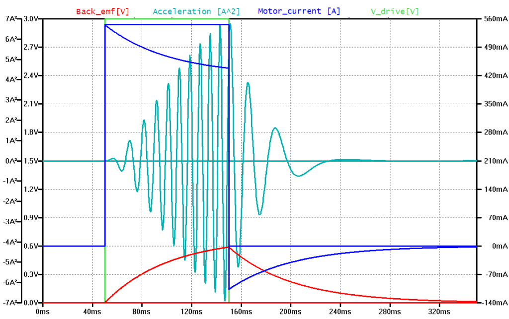
4) Stall Condition
To model a transient stall, simply use a voltage controlled switch in the mechanical path. Triggering the opening of this switch at a given time t effectively introduces infinite mechanical resistance.
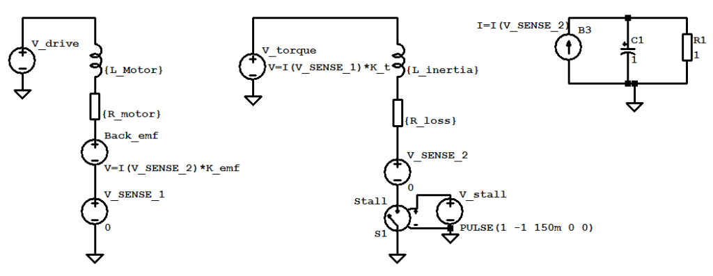
The “stall” switch is controlled by the voltage source V_stall. Example model parameters;
.model SW SW(Vt = 0.0 Ron = 1p)
.MODEL Stall SW(Vt = 0.01 Ron = 1n)
Make sure that Ron is set, as it defaults (in LTSpice) to 1 Ω, which is much greater than the mechanical circuit resistance. This is a general principle to be adhered to – when placing parts in the model, ensure you are aware of the component default values, don’t assume them to be zero.
Note that the 40ms between release and turn-off is insufficient for the back-EMF (red) to reach its maximum value. Note that it is also possible to model stall condition by using .STEP to perform parameter sweeps.
A Note On The .STEP Directive
The .STEP directive can be used to run sequential simulations with different component values. For example, to model a change in the rotor moment of inertia, simply vary the inertia of the mechanical equivalent circuit between two simulations as below:
.STEP param L_inertia .00000002 1.00000002 1
The STEP parameter above is used to run two simulations. The inductance of L_inertia is varied from .00000002 to 1.00000002 in steps of 1. This .STEP directive will, therefore, run two consecutive simulations.
The first simulation is a simple driving pulse of the duration of 100ms. The second run simulates a stall condition. This is modelled (using the .STEP directive) as a massive increase in L_inertia. Download here: DC MOTOR SPICE NETLIST
Conclusion
A SPICE model for a DC motor is presented. The model utilises a mechanical equivalent circuit to calculate the speed of the motor, taking into account the inertia and losses of the physical system. This is also used in determining the back EMF of the motor coils. Behavioural extensions to the model are presented, including a modification to model a stalled motor, inclusion of a gearbox, and finite turn-on voltage.
The complexity of the model required by a designer is application dependent. Once satisfied with the behaviour of the model, the designer can define a subcircuit (.SUBCKT) and create a simple two-wire symbol for the device.
For high-precision position systems, it will be necessary to improve the handling of friction in the model. Techniques such as the generalized Maxwell slip model (below) are well covered in the literature, and considered outside the scope of this bulletin.
References
- eCircuit Center, 2004, link
- Using Transformers in LTspice/SwitcherCAD III, Mike Engelhardt, Linear Technology Magazine, September 2006, link
- The Generalized Maxwell-Slip Model: A Novel Model for Friction Simulation and Compensation, Farid Al-Bender, Vincent Lampaert, and Jan Swevers, IEEE TRANSACTIONS ON AUTOMATIC CONTROL, VOL. 50, NO. 11, NOVEMBER 2005
Newsletter
Sign up to receive new blogs, case studies and resources – directly to your inbox.

Sign up
Discover more
Resources and guides
Discover our product application notes, design guides, news and case studies.
Case studies
Explore our collection of case studies, examples of our products in a range of applications.
Precision Microdrives
Whether you need a motor component, or a fully validated and tested complex mechanism – we’re here to help. Find out more about our company.